Semantic segmentation in rplatypus and pyplatypus: what is in the box

The last post took one published model and one dataset and asked where the model is weakest. This one steps back and opens the box: everything rplatypus and pyplatypus offer for semantic segmentation - a mask per class, scored by overlap - and how to choose among it all.

Training is what the package is for, and almost every field below is about training a model. To keep the post runnable on any laptop, its code only reads configurations and builds the networks, on the four nuclei images from the first post; the scores in it come from full training runs of the same configurations.

One file holds the experiment

Everything below can be passed to constructors in R or Python, but the clearest way to see it is the file both packages read. This one describes a whole training run:

nuclei.yaml

task: semantic_segmentation

data:
  train_path: nuclei
  validation_path: nuclei
  mode: nested_dirs
  colormap:
    - [0, 0, 0]          # background
    - [255, 255, 255]    # nucleus

models:
  - name: unet
    architecture: u_net
    input_shape: [256, 256]
    blocks: 4
    filters: 16
    loss:
      name: cce_dice
    metrics:
      - name: dice
        include_background: false
    optimizer:
      name: adam
      learning_rate: 0.001
    callbacks:
      - name: early_stopping
        monitor: val_dice
        patience: 5
    augmentation:
      - name: HorizontalFlip
        params: {p: 0.5}
      - name: RandomRotate90
        params: {p: 0.5}
    epochs: 30
    batch_size: 8

Read from the top:

task decides what the rest of the file may contain. Semantic segmentation is one of four; the others - classification, instance segmentation and object detection - get posts of their own.
data says where the images are and how to read them:
- train_path and validation_path say where the training and validation data are;
- mode is how the files are arranged: nested_dirs is one directory per image with images/ and masks/ inside, config_file is a CSV listing the files, which is what split_dataset() writes;
- colormap says which colour in a mask means which class, one entry per class, background first.
models is a list, so one file can train several models on the same data and compare them. Each entry has:
- a name, an architecture and an input_shape - these are required;
- blocks, the depth;
- filters, the width of the first block, doubling at each level down.
weights and fit are not in this file, because it trains from scratch:
- weights names a checkpoint - a published name from available_weights(), a Hugging Face reference or a local file - and training then starts from it rather than from random numbers;
- fit: false means no training at all: the weights are loaded and the model is ready for predict() and evaluate(), which is how the last post scored the published nuclei model.
loss, metrics, optimizer, callbacks and augmentation each take a name and that component’s own arguments. Every name comes from a catalogue the package can print, which is most of the rest of this post.

Reading it gives the same object as building it from arguments:

library(rplatypus)

spec <- platypus_spec("nuclei.yaml")
spec
#> platypus specification
#>   from        : nuclei.yaml 
#>   data        : nuclei 
#>   classes     : 2 
#>   models      : 1 
#>     unet           u_net            256x256, cce_dice, 30 epochs

import pyplatypus as pp

spec = pp.from_yaml("nuclei.yaml")
[(m.name, m.architecture.value, m.input_shape) for m in spec.models]
#> [('unet', 'u_net', (256, 256))]

The file is checked before a single image is read or the network is built, so a mistake costs a second rather than an epoch. Asking for something the architecture does not have is refused with the field that is wrong:

platypus_spec(
  data = segmentation_data("nuclei", "nuclei", colormap = binary_colormap),
  models = list(u_net("x", input_shape = c(256, 256),
                      deep_supervision = TRUE))
)
#> Error in `platypus_spec()`:
#> ! The specification has a problem:
#>   * models[[1]]: deep_supervision requires architecture 'u_net_plus_plus'; 'u_net' has no intermediate outputs to supervise

pp.from_dict({
    "task": "semantic_segmentation",
    "data": {"train_path": "nuclei", "validation_path": "nuclei",
             "colormap": [[0, 0, 0], [255, 255, 255]]},
    "models": [{"name": "x", "architecture": "u_net",
                "input_shape": [256, 256], "deep_supervision": True}],
})
#> ConfigError: The configuration has 1 problem:
#>   - models[0]: deep_supervision requires architecture 'u_net_plus_plus';
#>     'u_net' has no intermediate outputs to supervise

Four architectures

available_models(task = "semantic_segmentation")$name
#> [1] "u_net"           "u_net_plus_plus" "res_u_net"       "linknet"

[m["name"] for m in pp.available_models("semantic_segmentation")]
#> ['u_net', 'u_net_plus_plus', 'res_u_net', 'linknet']

All four are the same U: an encoder that halves the picture and doubles the features blocks times, and a decoder that climbs back up, with skip connections handing each level’s detail across. They differ in what is inside a block and in how the skips arrive.

Blue blocks are the encoder, green the decoder; each arrow is a connection. The picture going in is a stained tissue image from the same Data Science Bowl collection, and the one coming out is its true mask.

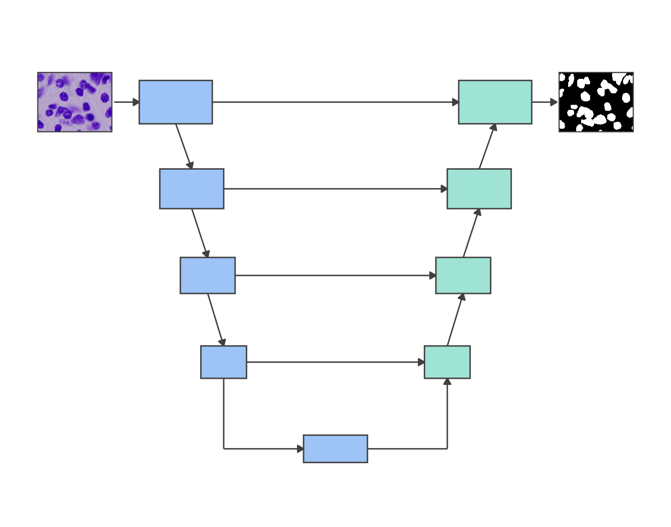
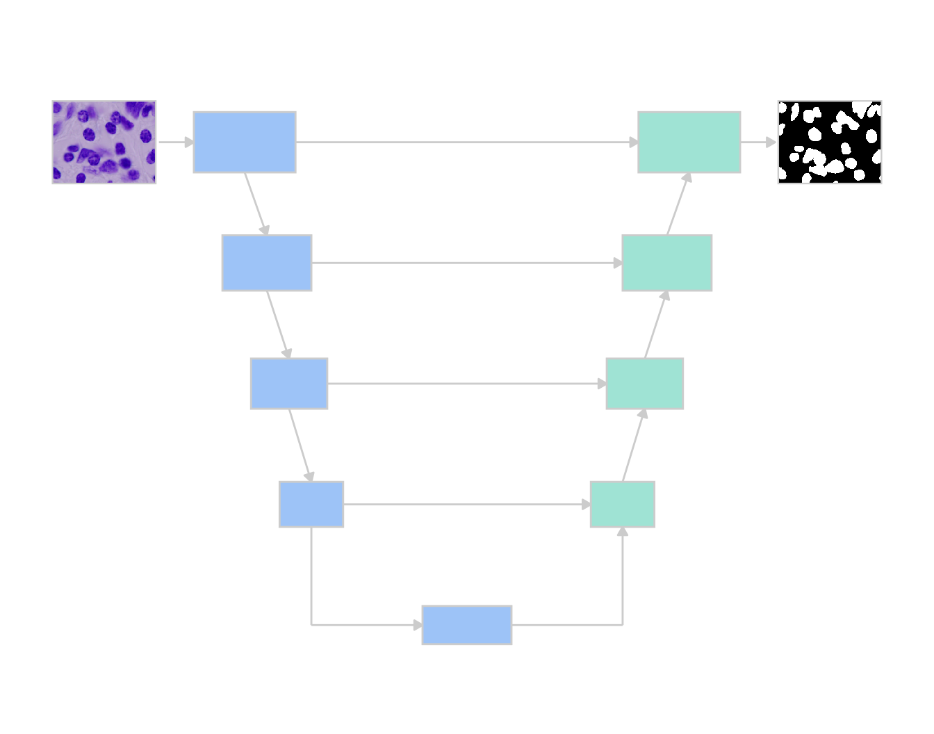
U-Net: each skip connection goes straight into the decoder block at the same level.

The plain U. Each skip connection is concatenated onto the decoder’s features, so a decoder block sees both what came up from below and what the encoder saw at its own scale. It is the one to start with.

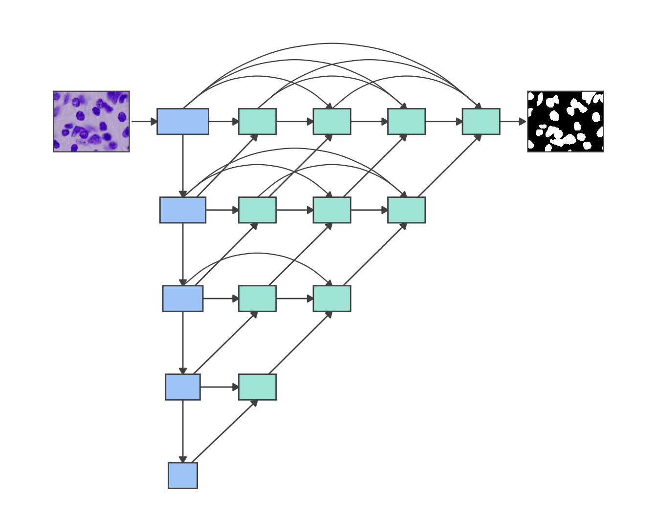
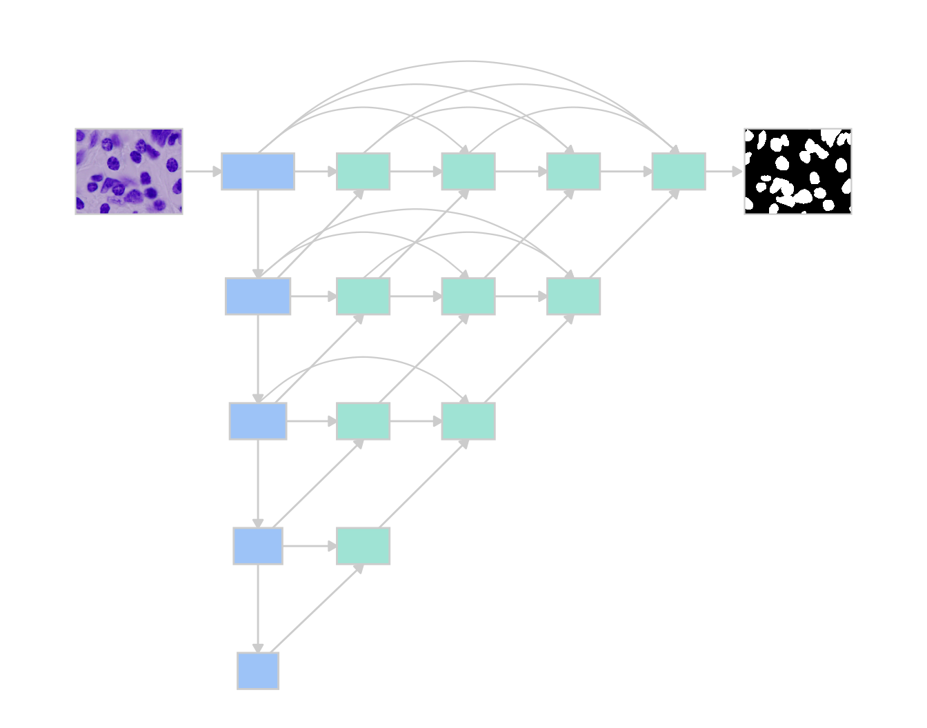
U-Net++: the space between encoder and decoder is filled with nested blocks, each fed by every earlier block in its row and by the one diagonally below.

The space between encoder and decoder is filled with nested blocks: each takes every earlier block in its row and the one diagonally below, so the top row - which is the decoder - meets the encoder at every depth rather than one. It is the only one of the four that can take deep_supervision, a loss on each block of the top row, which is the refusal above.

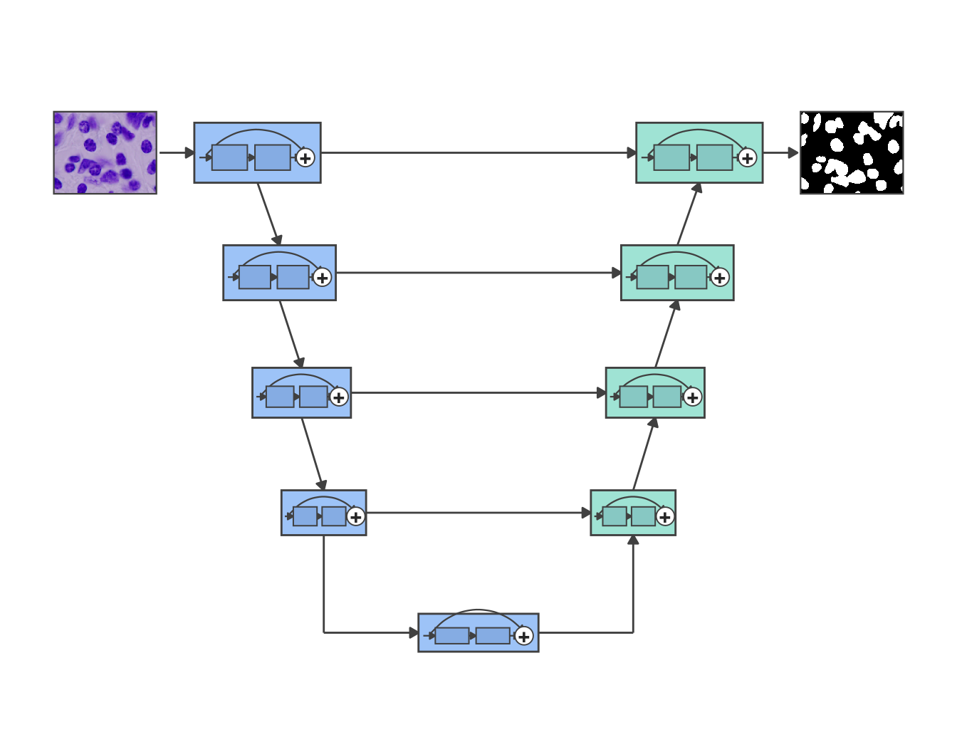
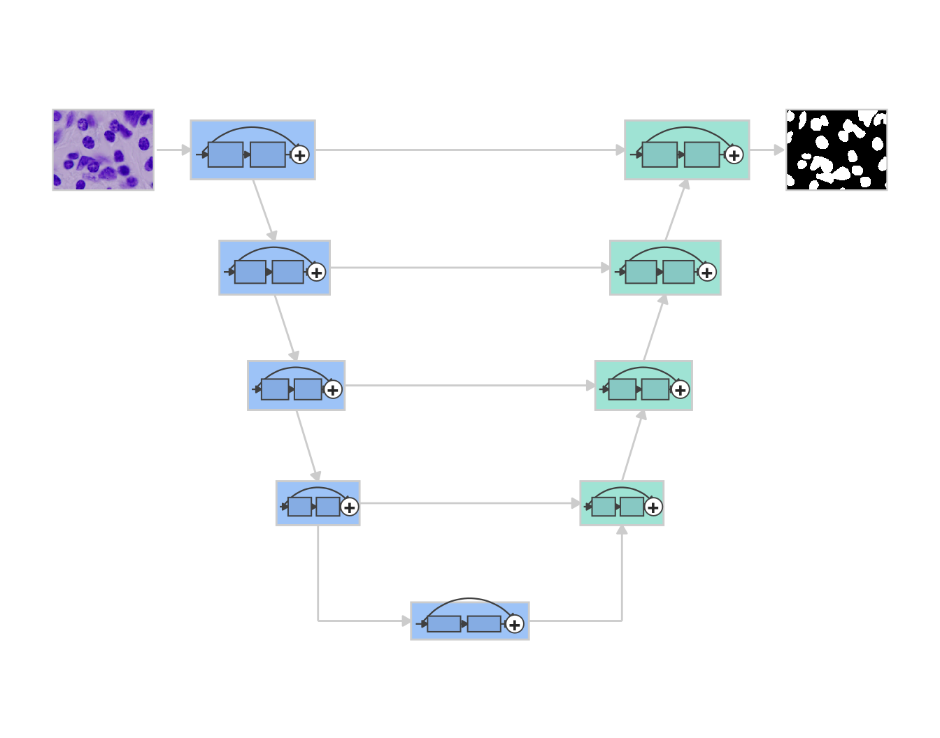
Res-U-Net: the U-Net layout with residual blocks - two layers and a shortcut over them, added back at the end.

The same U as U-Net, with residual blocks: each block’s input skips over its two layers and is added back at the end, so the layers learn a correction rather than a whole new representation. The usual reason to try it is depth, when more blocks stop helping.

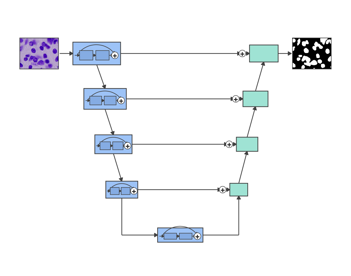
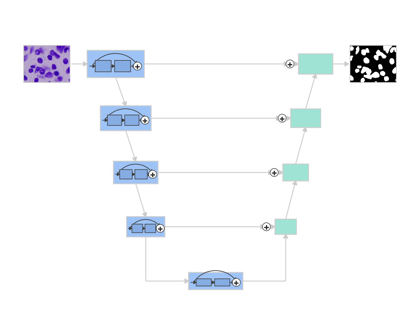
LinkNet: residual encoder blocks, skip connections added rather than concatenated, and a lighter decoder.

Residual blocks in the encoder, and skip connections that are added to the decoder’s features instead of concatenated onto them. Fewer channels reach each decoder block, so the decoder is lighter. Its argument is memory and speed, not score.

How much each costs at the same depth and width is quick to see. The cheapest way to build all four is one epoch on four small images:

one_epoch <- function(architecture, name) {
  architecture(name, input_shape = c(64, 64), blocks = 4, filters = 16,
               epochs = 1, batch_size = 2)
}
four <- platypus_spec(
  data = segmentation_data("nuclei", "nuclei", colormap = binary_colormap),
  models = list(one_epoch(u_net, "u_net"),
                one_epoch(u_net_plus_plus, "u_net_plus_plus"),
                one_epoch(res_u_net, "res_u_net"),
                one_epoch(linknet, "linknet"))
)
built <- platypus_fit(four, verbose = FALSE)
evaluate(built)[, c("model", "parameters")]
#>             model parameters
#> 1           u_net    1942594
#> 2 u_net_plus_plus    2263730
#> 3       res_u_net    2029682
#> 4         linknet    1746754

def one_epoch(architecture):
    return {"name": architecture, "architecture": architecture,
            "input_shape": [64, 64], "blocks": 4, "filters": 16,
            "epochs": 1, "batch_size": 2}

engine = pp.build_engine(pp.from_dict({
    "task": "semantic_segmentation",
    "data": {"train_path": "nuclei", "validation_path": "nuclei",
             "colormap": [[0, 0, 0], [255, 255, 255]]},
    "models": [one_epoch(a) for a in
               ["u_net", "u_net_plus_plus", "res_u_net", "linknet"]],
}))
engine.fit()
[(row["model"], row["parameters"]) for row in engine.evaluate()]
#> [('u_net', 1942594), ('u_net_plus_plus', 2263730),
#>  ('res_u_net', 2029682), ('linknet', 1746754)]

LinkNet is 10% smaller than U-Net here, not half: at 16 filters and four blocks the shared skeleton dominates, and the decoder savings are a small part of it.

Which one wins

When the nuclei weights were published, all four were trained on the same split of the 2018 Data Science Bowl images, with the same specification, for 60 epochs:

architecture	parameters	mean Dice
U-Net	1,942,594	0.9217
U-Net++	2,263,730	0.9212
LinkNet	1,746,754	0.9203
Res-U-Net	2,029,682	0.9187

The four means are 0.0030 apart. Within any one of them, the images it was scored on are 0.054 apart. And training the same U-Net again with a different seed moved its mean by 0.0012 - 40% of the whole gap between architectures.

On this problem the architecture is not where the result comes from, and that is why only one set of weights was published rather than four. It will not be true of every dataset, but it is the reason to start with a plain U-Net and look for a gain somewhere else first - the data, the loss, the resolution - before swapping the network.

Losses and metrics

available_losses(task = "semantic_segmentation")$name
#>  [1] "boundary"         "cce"              "cce_dice"        
#>  [4] "combo"            "dice"             "focal"           
#>  [7] "focal_tversky"    "generalized_dice" "iou"             
#> [10] "lovasz"           "tversky"
available_metrics(task = "semantic_segmentation")$name
#> [1] "cldice"       "dice"         "iou"          "surface_dice"
#> [5] "tversky"

[l["name"] for l in pp.available_losses("semantic_segmentation")]
#> ['boundary', 'cce', 'cce_dice', 'combo', 'dice', 'focal', 'focal_tversky',
#>  'generalized_dice', 'iou', 'lovasz', 'tversky']
[m["name"] for m in pp.available_metrics("semantic_segmentation")]
#> ['cldice', 'dice', 'iou', 'surface_dice', 'tversky']

The task matters here: classification, detection and instance segmentation each have their own architectures, losses and metrics, and the same functions list them. Each entry also comes with its arguments and a one-line description. The short version of the losses:

cce_dice - cross-entropy blended with Dice - is the one to start a run with.
tversky and focal_tversky take an alpha that weighs a missed pixel against a false alarm. Above 0.5 they would rather over-segment than miss, which suits a small class you cannot afford to lose.
generalized_dice weights each class by the inverse square of its area, so with several classes of very different size the small ones still count.
boundary adds a term for how far a wrong pixel is from the true edge, and lovasz optimises the IoU you are going to report rather than a stand-in for it.

The metrics are fewer and each answers a different question. dice is the one to report unless there is a reason not to - with include_background = FALSE, as the last post explained. cldice asks whether a thin structure stays connected, which a vessel post later in the series needs, and surface_dice asks how much of a boundary lies within a tolerance of the truth, which matters for volumes.

Training, around the model

The rest of the file is the training run itself, and each part has its catalogue too:

available_optimizers()$name
#> [1] "adadelta" "adagrad"  "adam"     "adamax"   "adamw"    "nadam"   
#> [7] "rmsprop"  "sgd"
available_callbacks()$name
#>  [1] "cosine_annealing"      "csv_logger"            "early_stopping"       
#>  [4] "ema"                   "linear_annealing"      "model_checkpoint"     
#>  [7] "reduce_lr_on_plateau"  "step_decay"            "stop_after"           
#> [10] "swa"                   "terminate_on_collapse" "terminate_on_nan"
length(available_transforms())
#> [1] 118

[o["name"] for o in pp.available_optimizers()]
#> ['adadelta', 'adagrad', 'adam', 'adamax', 'adamw', 'nadam', 'rmsprop',
#>  'sgd']
[c["name"] for c in pp.available_callbacks()]
#> ['cosine_annealing', 'csv_logger', 'early_stopping', 'ema',
#>  'linear_annealing', 'model_checkpoint', 'reduce_lr_on_plateau',
#>  'step_decay', 'stop_after', 'swa', 'terminate_on_collapse',
#>  'terminate_on_nan']
len(pp.available_transforms())
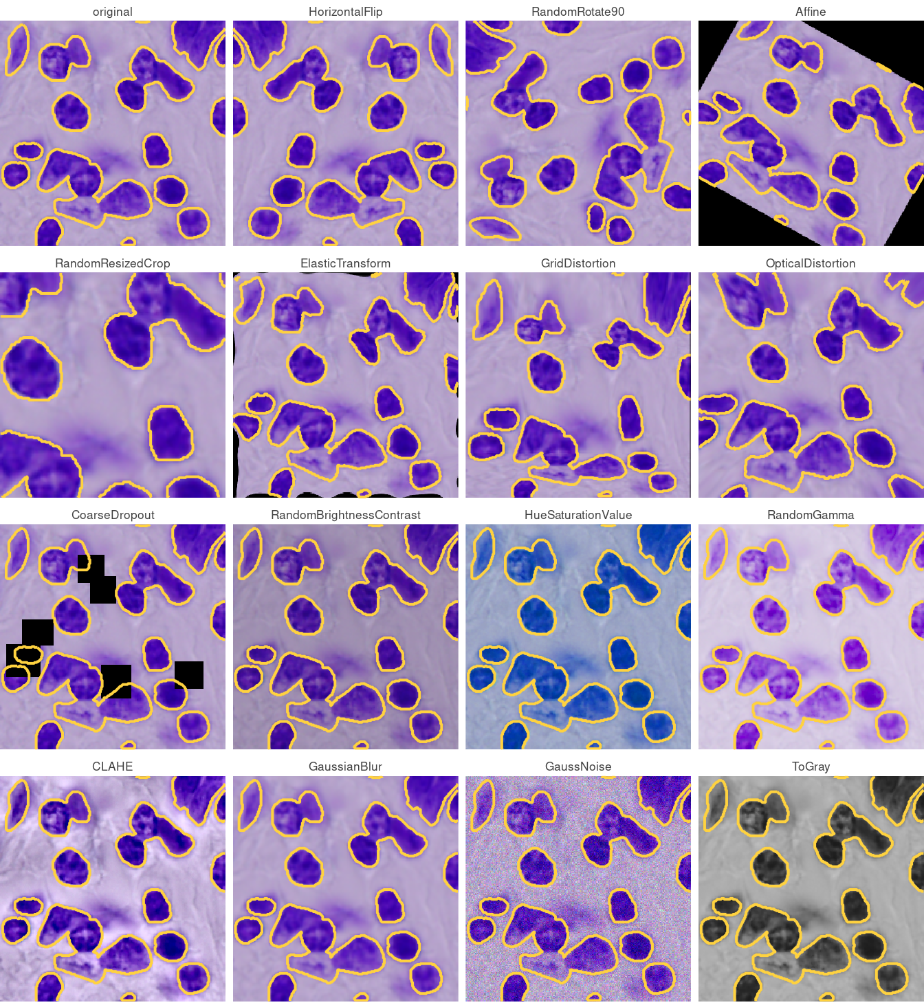
#> 118

Eight optimisers; twelve callbacks, from early stopping and learning-rate schedules to weight averaging (ema, swa) and two that stop a run that has gone wrong rather than letting it finish; and 118 augmentations from albumentations, each named exactly as albumentations names it, with its own parameters under params.

Fifteen of them, on the image from the architecture diagrams, each applied every time (p = 1); the yellow line is the mask that comes out with it. The ones that move pixels around move the mask with the image, and the ones that change colour, contrast or sharpness leave it where it was:

The original image and fifteen albumentations transforms. Yellow: the outline of the mask after each transform.

Big images: tiles instead of shrinking

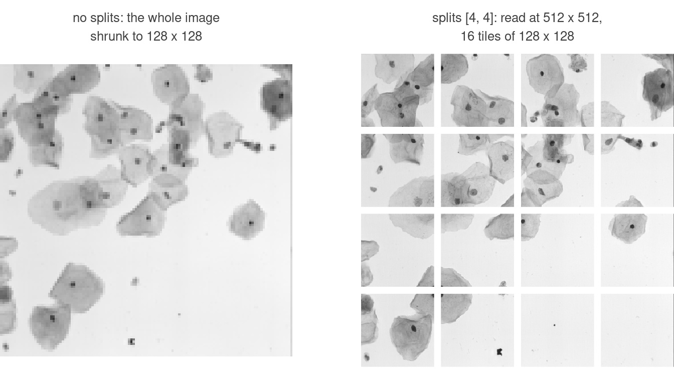
Every image is resized to input_shape before the network sees it. The nuclei lose little that way, which is why nuclei.yaml has no splits, but a 1024-pixel image shrunk to 128 keeps a nucleus as a few pixels. splits cuts the image into a grid of tiles instead, one number per spatial dimension:

models:
  - name: tiled
    architecture: u_net
    input_shape: [128, 128]     # what the network sees: one tile
    splits: [4, 4]              # 4 rows x 4 columns
    batch_size: 2

The constructors take the same field:

tiled <- u_net("tiled", input_shape = c(128, 128), splits = c(4, 4),
               blocks = 4, filters = 16, batch_size = 2, epochs = 40)
platypus_spec(
  data = segmentation_data("nuclei", "nuclei", colormap = binary_colormap),
  models = list(tiled)
)
#> platypus specification
#>   data        : nuclei 
#>   classes     : 2 
#>   models      : 1 
#>     tiled          u_net            128x128, tiled 4x4, cce, 40 epochs

tiled = {"name": "tiled", "architecture": "u_net",
         "input_shape": [128, 128], "splits": [4, 4],
         "blocks": 4, "filters": 16, "batch_size": 2, "epochs": 40}
spec = pp.from_dict({
    "task": "semantic_segmentation",
    "data": {"train_path": "nuclei", "validation_path": "nuclei",
             "colormap": [[0, 0, 0], [255, 255, 255]]},
    "models": [tiled],
})
m = spec.models[0]
m.load_shape, m.tiles_per_image
#> ((512, 512), 16)

input_shape is still what the network sees, which is now one tile. The image is read at splits times that and cut, so one source image gives as many training samples as there are tiles:

splits	image read at	tiles per image
not set	128 x 128	1
`[2, 3]`	256 x 384	6
`[4, 4]`	512 x 512	16

One 1024 x 1024 image from the nuclei data as a network with input_shape 128 x 128 gets it: shrunk without splits, cut into sixteen tiles with splits [4, 4].

Three things follow:

The source image does not have to be a multiple of the tile: it is resized to the size it is read at - 1024 x 1024 to 512 x 512 above, and a 696 x 520 image to the same square - and only then cut. The tile has the rule it had without tiling: every block halves it, so with blocks = 4 each side of input_shape must divide by 16. A tile of 127 x 127 is refused when the file is read: every spatial dimension must be divisible by 16; input_shape=(127, 127) is not.
predict() puts the tiles back together, so it returns one mask per image at its original size rather than sixteen pieces.
cldice and surface_dice are properties of a whole mask, not of a tile, so a tiled run does not report them per epoch; evaluate_cases() scores them per image afterwards. A callback that watches one of them on a tiled run is refused when the file is read.

The series so far

rplatypus rebuilt: deep learning for medical images in R - why the 2020 package had to be rewritten, how it now installs its own Python, and a first mask from published weights.
Nuclei, five years later - a mean Dice of 0.92, and the three images it hides.
Semantic segmentation in rplatypus and pyplatypus: what is in the box - this post.

The next one leaves segmentation for classification, where the number that hides things is not a mean but an accuracy: a classifier at 0.97 that has learnt nothing at all.