
Explainable Artificial Intelligence, or XAI for short, is a set of tools that helps us understand and interpret complicated “black box” machine and deep learning models and their predictions. In my previous post I showed you a sneak peek of my newest package called sauron, which allows you to explain decisions of Convolutional Neural Networks. I am really glad to say that beta version of sauron is finally here!
Sauron
With sauron you can use Explainable Artificial Intelligence (XAI) methods to understand predictions made by Neural Networks in tensorflow/keras. For the time being only Convolutional Neural Networks are supported, but it will change in time.
You can install the latest version of sauron with remotes:
remotes::install_github("maju116/sauron")Note that in order to install platypus you need to install keras and tensorflow packages and Tensorflow version >= 2.0.0 (Tensorflow 1.x will not be supported!)
Quick example: How it all works?
To generate any explanations you will have to create an object of class CNNexplainer. To do this you will need two things:
- tensorflow/keras model
- image preprocessing function (optional)
library(tidyverse)
library(sauron)

model <- application_xception()
preprocessing_function <- xception_preprocess_input

explainer <- CNNexplainer$new(model = model,
                              preprocessing_function = preprocessing_function,
                              id = "imagenet_xception")
explainer
# <CNNexplainer>
#   Public:
#     clone: function (deep = FALSE)
#     explain: function (input_imgs_paths, class_index = NULL, methods = c("V",
#     id: imagenet_xception
#     initialize: function (model, preprocessing_function, id = NULL)
#     model: function (object, ...)
#     preprocessing_function: function (x)
#     show_available_methods: function ()
#   Private:
#     available_methods: tbl_df, tbl, data.frame
To see available XAI methods for the CNNexplainer object use:
explainer$show_available_methods()
# # A tibble: 8 x 2
#   method name
#   <chr>  <chr>
# 1 V      Vanilla gradient
# 2 GI     Gradient x Input
# 3 SG     SmoothGrad
# 4 SGI    SmoothGrad x Input
# 5 IG     Integrated Gradients
# 6 GB     Guided Backpropagation
# 7 OCC    Occlusion Sensitivity
# 8 GGC    Guided Grad-CAM
Now you can explain predictions using explain method. You will need:
- paths to the images for which you want to generate explanations.
- class indexes for which the explanations should be generated (optional, if set to
NULLclass that maximizes predicted probability will be found for each image). - character vector with method names (optional, by default explainer will use all methods).
- batch size (optional, by default number of inserted images).
- additional arguments with settings for a specific method (optional).
As an output you will get an object of class CNNexplanations:
input_imgs_paths <- list.files(system.file("extdata", "images", package = "sauron"), full.names = TRUE)

explanations <- explainer$explain(input_imgs_paths = input_imgs_paths,
                                  class_index = NULL,
                                  batch_size = 1,
                                  methods = c("V", "IG",  "GB", "GGC"),
                                  steps = 10, # Number of Integrated Gradients steps
                                  grayscale = FALSE # RGB or Gray gradients
)

explanations
# CNNexplanations object contains explanations for 3 images for 1 model.
You can get raw explanations and metadata from CNNexplanations object using:
explanations$get_metadata()
# $multimodel_explanations
# [1] FALSE
#
# $ids
# [1] "imagenet_xception"
#
# $n_models
# [1] 1
#
# $target_sizes
# $target_sizes[[1]]
# [1] 299 299 3
#
#
# $methods
# [1] "V" "IG" "GB" "GGC"
#
# $input_imgs_paths
# [1] "/home/maju116/R/x86_64-pc-linux-gnu-library/4.0/sauron/extdata/images/cat_and_dog.jpg"
# [2] "/home/maju116/R/x86_64-pc-linux-gnu-library/4.0/sauron/extdata/images/cat.jpeg"
# [3] "/home/maju116/R/x86_64-pc-linux-gnu-library/4.0/sauron/extdata/images/zebras.jpg"
#
# $n_imgs
# [1] 3
raw_explanations <- explanations$get_explanations()
str(raw_explanations)
# List of 1
# $ imagenet_xception:List of 5
# ..$ Input: num [1:3, 1:299, 1:299, 1:3] 147 134 170 147 134 168 144 134 170 144 ...
# .. ..- attr(*, "dimnames")=List of 4
# .. .. ..$ : NULL
# .. .. ..$ : NULL
# .. .. ..$ : NULL
# .. .. ..$ : NULL
# ..$ V : int [1:3, 1:299, 1:299, 1:3] 0 0 0 0 0 0 0 0 0 0 ...
# .. ..- attr(*, "dimnames")=List of 4
# .. .. ..$ : NULL
# .. .. ..$ : NULL
# .. .. ..$ : NULL
# .. .. ..$ : NULL
# ..$ IG : int [1:3, 1:299, 1:299, 1:3] 0 0 0 0 0 0 0 0 0 0 ...
# .. ..- attr(*, "dimnames")=List of 4
# .. .. ..$ : NULL
# .. .. ..$ : NULL
# .. .. ..$ : NULL
# .. .. ..$ : NULL
# ..$ GB : int [1:3, 1:299, 1:299, 1:3] 0 0 2 0 0 111 0 0 28 0 ...
# .. ..- attr(*, "dimnames")=List of 4
# .. .. ..$ : NULL
# .. .. ..$ : NULL
# .. .. ..$ : NULL
# .. .. ..$ : NULL
# ..$ GGC : num [1:3, 1:299, 1:299, 1] 7.13e-05 0.00 4.55e-04 7.13e-05 0.00 ...
# .. ..- attr(*, "dimnames")=List of 4
# .. .. ..$ : NULL
# .. .. ..$ : NULL
# .. .. ..$ : NULL
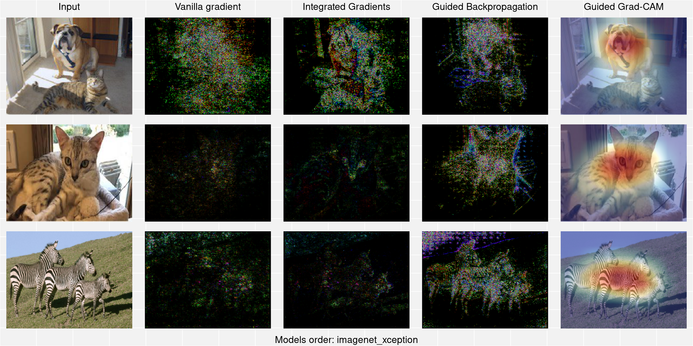
# .. .. ..$ : NULLTo visualize and save generated explanations use:
explanations$plot_and_save(combine_plots = TRUE, # Show all explanations side by side on one image?
                           output_path = NULL, # Where to save output(s)
                           plot = TRUE # Should output be plotted?
)
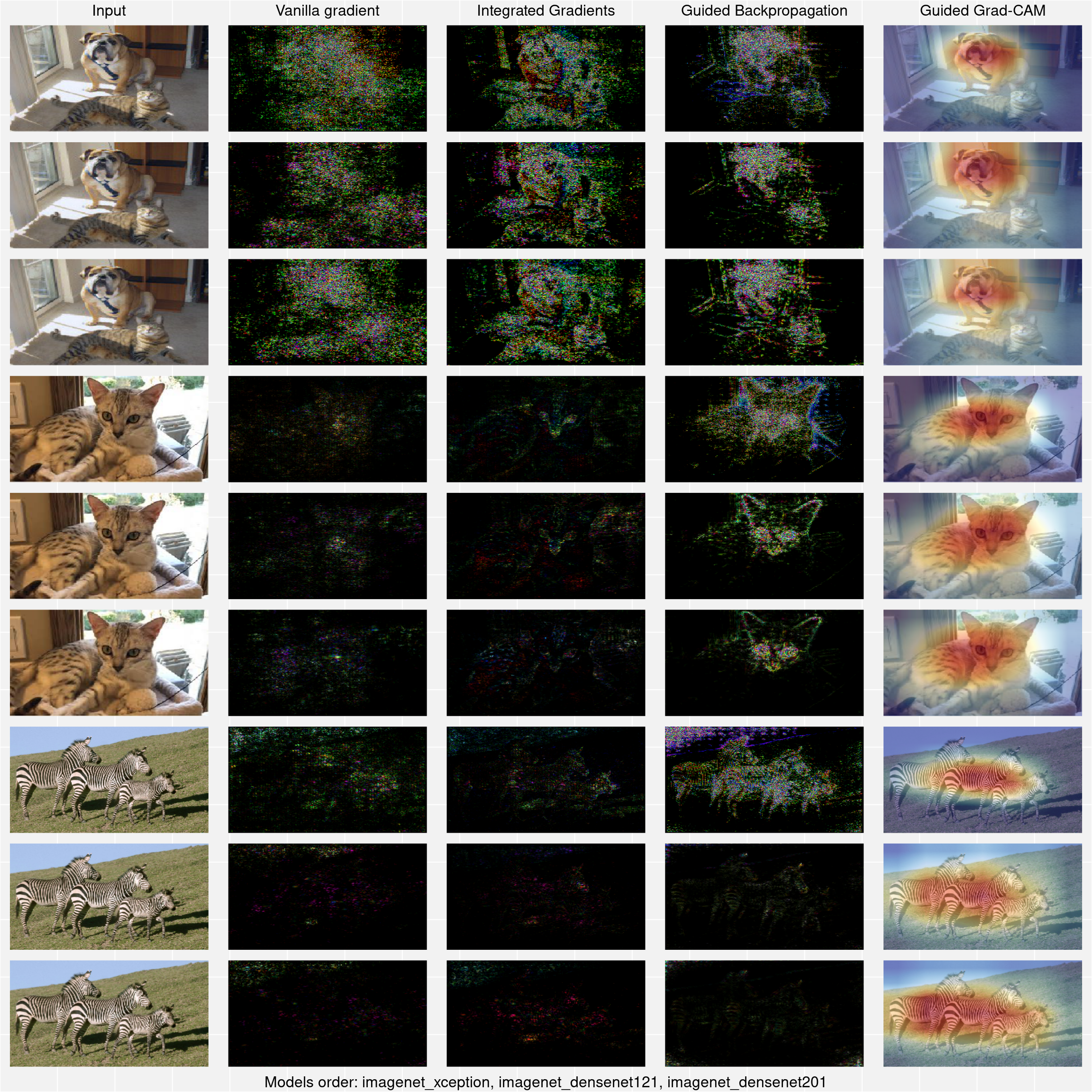
If you want to compare two or more different models you can do it by combining CNNexplainer objects into CNNexplainers object:
model2 <- application_densenet121()
preprocessing_function2 <- densenet_preprocess_input

explainer2 <- CNNexplainer$new(model = model2,
                               preprocessing_function = preprocessing_function2,
                               id = "imagenet_densenet121")

model3 <- application_densenet201()
preprocessing_function3 <- densenet_preprocess_input

explainer3 <- CNNexplainer$new(model = model3,
                               preprocessing_function = preprocessing_function3,
                               id = "imagenet_densenet201")

explainers <- CNNexplainers$new(explainer, explainer2, explainer3)

explanations123 <- explainers$explain(input_imgs_paths = input_imgs_paths,
                                      class_index = NULL,
                                      batch_size = 1,
                                      methods = c("V", "IG",  "GB", "GGC"),
                                      steps = 10,
                                      grayscale = FALSE
)

explanations123$get_metadata()
# $multimodel_explanations
# [1] TRUE
#
# $ids
# [1] "imagenet_xception"    "imagenet_densenet121" "imagenet_densenet201"
#
# $n_models
# [1] 3
#
# $target_sizes
# $target_sizes[[1]]
# [1] 299 299   3
#
# $target_sizes[[2]]
# [1] 224 224   3
#
# $target_sizes[[3]]
# [1] 224 224   3
#
#
# $methods
# [1] "V"   "IG"  "GB"  "GGC"
#
# $input_imgs_paths
# [1] "/home/maju116/R/x86_64-pc-linux-gnu-library/4.0/sauron/extdata/images/cat_and_dog.jpg"
# [2] "/home/maju116/R/x86_64-pc-linux-gnu-library/4.0/sauron/extdata/images/cat.jpeg"
# [3] "/home/maju116/R/x86_64-pc-linux-gnu-library/4.0/sauron/extdata/images/zebras.jpg"
#
# $n_imgs
# [1] 3

explanations123$plot_and_save(combine_plots = TRUE,
                              output_path = NULL,
                              plot = TRUE
)
Alternatively if you already have some CNNexplanations objects generated (for the same images and using same methods) you can combine them:
explanations2 <- explainer2$explain(input_imgs_paths = input_imgs_paths,
                                    class_index = NULL,
                                    batch_size = 1,
                                    methods = c("V", "IG",  "GB", "GGC"),
                                    steps = 10,
                                    grayscale = FALSE
)

explanations3 <- explainer3$explain(input_imgs_paths = input_imgs_paths,
                                    class_index = NULL,
                                    batch_size = 1,
                                    methods = c("V", "IG",  "GB", "GGC"),
                                    steps = 10,
                                    grayscale = FALSE
)

explanations$combine(explanations2, explanations3)

explanations$get_metadata()
# $multimodel_explanations
# [1] TRUE
#
# $ids
# [1] "imagenet_xception"    "imagenet_densenet121" "imagenet_densenet201"
#
# $n_models
# [1] 3
#
# $target_sizes
# $target_sizes[[1]]
# [1] 299 299   3
#
# $target_sizes[[2]]
# [1] 224 224   3
#
# $target_sizes[[3]]
# [1] 224 224   3
#
#
# $methods
# [1] "V"   "IG"  "GB"  "GGC"
#
# $input_imgs_paths
# [1] "/home/maju116/R/x86_64-pc-linux-gnu-library/4.0/sauron/extdata/images/cat_and_dog.jpg"
# [2] "/home/maju116/R/x86_64-pc-linux-gnu-library/4.0/sauron/extdata/images/cat.jpeg"
# [3] "/home/maju116/R/x86_64-pc-linux-gnu-library/4.0/sauron/extdata/images/zebras.jpg"
#
# $n_imgs
# [1] 3

explanations$plot_and_save(combine_plots = TRUE,
                           output_path = NULL,
                           plot = TRUE
)
