Computer Vision tasks
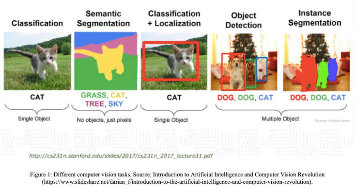
Computer Vision, or CV for short, is a field of computer science focused on development of techniques that will help computers understand the content of digital images in a way similar to human understanding. There’s a lot of different computer vision tasks, but today I want to focus only on four basic ones.

Basic Computer Vision tasks:
- Image classification - in this task we want to compute the probability (or probabilities) that the input image is in a particular class. It could be performed with Convolutional Neural Networks using
keraspackage. - Semantic segmentation - very similar to image classification, but instead of classifying the whole image, we want to classify each pixel of this image. Note that we are not saying anything about location of the object.
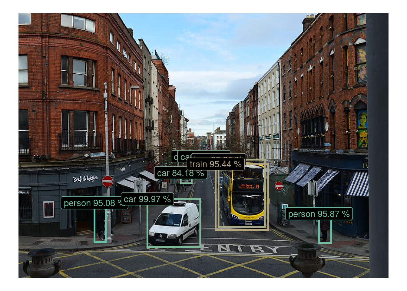
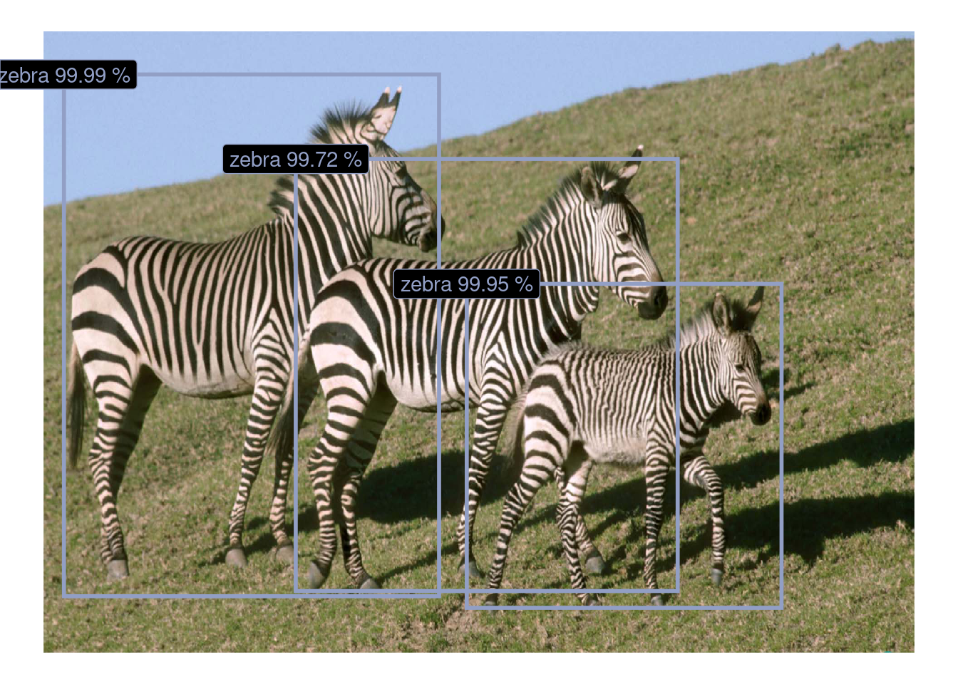
- Object detection - we want to classify and locate objects on the input image. Object localization is typically indicated by specifying a tightly cropped bounding box.
- Instance segmentation - it’s a combination of semantic segmentation and object detection. Like in semantic segmentation we want to classify each pixel to a different class, but we also want to distinguish between different objects of the same class.
Platypus
platypus is an R package for object detection and semantic segmentation. Currently using platypus you can perform:
- multi-class semantic segmentation using U-Net architecture
- multi-class object detection using YOLOv3 architecture
You can install the latest version of platypus with remotes package:
remotes::install_github("maju116/platypus")Note that in order to install platypus you need to install keras and tensorflow packages and Tensorflow version >= 2.0.0 (Tensorflow 1.x will not be supported!)
Quick example: YOLOv3 bounding box prediction with pre-trained COCO weights
To create YOLOv3 architecture use:
library(tidyverse)
library(platypus)
library(abind)

test_yolo <- yolo3(
  net_h = 416, # Input image height. Must be divisible by 32
  net_w = 416, # Input image width. Must be divisible by 32
  grayscale = FALSE, # Should images be loaded as grayscale or RGB
  n_class = 80, # Number of object classes (80 for COCO dataset)
  anchors = coco_anchors # Anchor boxes
)

test_yolo
#> Model
#> Model: "yolo3"
#> ________________________________________________________________________________
#> Layer (type)              Output Shape      Param #  Connected to
#> ================================================================================
#> input_img (InputLayer)    [(None, 416, 416, 0
#> ________________________________________________________________________________
#> darknet53 (Model)         multiple          40620640 input_img[0][0]
#> ________________________________________________________________________________
#> yolo3_conv1 (Model)       (None, 13, 13, 51 11024384 darknet53[1][2]
#> ________________________________________________________________________________
#> yolo3_conv2 (Model)       (None, 26, 26, 25 2957312  yolo3_conv1[1][0]
#>                                                      darknet53[1][1]
#> ________________________________________________________________________________
#> yolo3_conv3 (Model)       (None, 52, 52, 12 741376   yolo3_conv2[1][0]
#>                                                      darknet53[1][0]
#> ________________________________________________________________________________
#> grid1 (Model)             (None, 13, 13, 3, 4984063  yolo3_conv1[1][0]
#> ________________________________________________________________________________
#> grid2 (Model)             (None, 26, 26, 3, 1312511  yolo3_conv2[1][0]
#> ________________________________________________________________________________
#> grid3 (Model)             (None, 52, 52, 3, 361471   yolo3_conv3[1][0]
#> ================================================================================
#> Total params: 62,001,757
#> Trainable params: 61,949,149
#> Non-trainable params: 52,608
#> ________________________________________________________________________________
You can now load YOLOv3 Darknet weights trained on COCO dataset. Download pre-trained weights from here and run:
test_yolo %>% load_darknet_weights("yolov3.weights")Calculate predictions for new images:
test_img_paths <- list.files(system.file("extdata", "images", package = "platypus"), full.names = TRUE, pattern = "coco")
test_imgs <- test_img_paths %>%
  map(~ {
    image_load(., target_size = c(416, 416), grayscale = FALSE) %>%
      image_to_array() %>%
      `/`(255)
  }) %>%
  abind(along = 4) %>%
  aperm(c(4, 1:3))
test_preds <- test_yolo %>% predict(test_imgs)

str(test_preds)
#> List of 3
#>  $ : num [1:2, 1:13, 1:13, 1:3, 1:85] 0.294 0.478 0.371 1.459 0.421 ...
#>  $ : num [1:2, 1:26, 1:26, 1:3, 1:85] -0.214 1.093 -0.092 2.034 -0.286 ...
#>  $ : num [1:2, 1:52, 1:52, 1:3, 1:85] 0.242 -0.751 0.638 -2.419 -0.282 ...
Transform raw predictions into bounding boxes:
test_boxes <- get_boxes(
  preds = test_preds, # Raw predictions form YOLOv3 model
  anchors = coco_anchors, # Anchor boxes
  labels = coco_labels, # Class labels
  obj_threshold = 0.6, # Object threshold
  nms = TRUE, # Should non-max suppression be applied
  nms_threshold = 0.6, # Non-max suppression threshold
  correct_hw = FALSE # Should height and width of bounding boxes be corrected to image height and width
)

test_boxes
#> [[1]]
#> # A tibble: 8 x 7
#>    xmin  ymin  xmax  ymax p_obj label_id label
#>   <dbl> <dbl> <dbl> <dbl> <dbl>    <int> <chr>
#> 1 0.207 0.718 0.236 0.865 0.951        1 person
#> 2 0.812 0.758 0.846 0.868 0.959        1 person
#> 3 0.349 0.702 0.492 0.884 1.00         3 car
#> 4 0.484 0.543 0.498 0.558 0.837        3 car
#> 5 0.502 0.543 0.515 0.556 0.821        3 car
#> 6 0.439 0.604 0.469 0.643 0.842        3 car
#> 7 0.541 0.554 0.667 0.809 0.999        6 bus
#> 8 0.534 0.570 0.675 0.819 0.954        7 train
#>
#> [[2]]
#> # A tibble: 3 x 7
#>     xmin   ymin  xmax  ymax p_obj label_id label
#>    <dbl>  <dbl> <dbl> <dbl> <dbl>    <int> <chr>
#> 1 0.0236 0.0705 0.454 0.909 1.00        23 zebra
#> 2 0.290  0.206  0.729 0.901 0.997       23 zebra
#> 3 0.486  0.407  0.848 0.928 1.00        23 zebra
Plot / save images:
plot_boxes(
  images_paths = test_img_paths, # Images paths
  boxes = test_boxes, # Bounding boxes
  correct_hw = TRUE, # Should height and width of bounding boxes be corrected to image height and width
  labels = coco_labels # Class labels
)

For more details and examples on custom datasets visit platypus page and check out the latest posts.