The data

Today we will work on 2018 Data Science Bowl dataset. You can download images and masks directly form the url or using Kagge API :

kaggle competitions download -c data-science-bowl-2018

After downloading the data, unpack them and move to preferred destination. For this example we will be interested only in stage1_train and stage1_test subdirectories, so you can delete other files if you want.

Before we start, let’s investigate a little bit.

library(tidyverse)
library(platypus)
library(abind)
library(here)

# Print current working directory
here()

# [1] "/home/maju116/Desktop/PROJECTS/Moje Projekty/platypus"

# Set directories with the data and models
data_path <- here("examples/data/data-science-bowl-2018/")
models_path <- here("examples/models/")

# Investigate one instance of data (image + masks)
sample_image_path <- here("examples/data/data-science-bowl-2018/stage1_train/00071198d059ba7f5914a526d124d28e6d010c92466da21d4a04cd5413362552/")

list.files(sample_image_path, full.names = TRUE) %>%
  set_names(basename(.)) %>%
  map(~ list.files(.))

# $images
# [1] "00071198d059ba7f5914a526d124d28e6d010c92466da21d4a04cd5413362552.png"
# 
# $masks
#  [1] "07a9bf1d7594af2763c86e93f05d22c4d5181353c6d3ab30a345b908ffe5aadc.png"
#  [2] "0e548d0af63ab451616f082eb56bde13eb71f73dfda92a03fbe88ad42ebb4881.png"
#  [3] "0ea1f9e30124e4aef1407af239ff42fd6f5753c09b4c5cac5d08023c328d7f05.png"
#  [4] "0f5a3252d05ecdf453bdd5e6ad5322c454d8ec2d13ef0f0bf45a6f6db45b5639.png"
#  [5] "2c47735510ef91a11fde42b317829cee5fc04d05a797b90008803d7151951d58.png"
#  [6] "4afa39f2a05f9884a5ff030d678c6142379f99a5baaf4f1ba7835a639cb50751.png"
#  [7] "4bc58dbdefb2777392361d8b2d686b1cc14ca310e009b79763af46e853e6c6ac.png"
#  [8] "4e3b49fb14877b63704881a923365b68c1def111c58f23c66daa49fef4b632bf.png"
#  [9] "5522143fa8723b66b1e0b25331047e6ae6eeec664f7c8abeba687e0de0f9060a.png"
# [10] "58656859fb9c13741eda9bc753c3415b78d1135ee852a194944dee88ab70acf4.png"
# [11] "6442251746caac8fc255e6a22b41282ffcfabebadbd240ee0b604808ff9e3383.png"
# [12] "7ff04129f8b6d9aaf47e062eadce8b3fcff8b4a29ec5ad92bca926ac2b7263d2.png"
# [13] "8bbec3052bcec900455e8c7728d03facb46c880334bcc4fb0d1d066dd6c7c5d2.png"
# [14] "9576fe25f4a510f12eecbabfa2e0237b98d8c2622b9e13b9a960e2afe6da844e.png"
# [15] "95deddb72b845b1a1f81a282c86e666045da98344eaa2763d67e2ab80bc2e5c3.png"
# [16] "a1b0cdb21f341af17d86f23596df4f02a6b9c4e0d59a7f74aaf28b9e408a4e4c.png"
# [17] "aa154c70e0d82669e9e492309bd00536d2b0f6eeec1210014bbafbfc554b377c.png"
# [18] "acba6646e8250aab8865cd652dfaa7c56f643267ea2e774aee97dc2342d879d6.png"
# [19] "ae00049dc36a1e5ffafcdeadb44b18a9cd6dfd459ee302ab041337529bd41cf2.png"
# [20] "af4d6ff17fa7b41de146402e12b3bab1f1fe3c1e6f37da81a54e002168b1e7dd.png"
# [21] "b0cbc2c553f9c4ac2191395236f776143fb3a28fb77b81d3d258a2f45361ca89.png"
# [22] "b6fc3b5403de8f393ca368553566eaf03d5c07148539bc6141a486f1d185f677.png"
# [23] "be98de8a7ba7d5d733b1212ae957f37b5b69d0bf350b9a5a25ba4346c29e49f7.png"
# [24] "cb53899ef711bce04b209829c61958abdb50aa759f3f896eb7ed868021c22fb4.png"
# [25] "d5024b272cb39f9ef2753e2f31344f42dd17c0e2311c4927946bc5008d295d2e.png"
# [26] "f6eee5c69f54807923de1ceb1097fc3aa902a6b20d846f111e806988a4269ed0.png"
# [27] "ffae764df84788e8047c0942f55676c9663209f65da943814c6b3aca78d8e7f7.png"

As you can see each image has its own directory, that has two subdirectories inside:

• images - contains original image that will be the input of the neural network
• masks - contains one or more segmentation masks. Segmentation mask is simply telling us which pixel belongs to which class, and this is what we will try to predict.

For the modeling, beside train and test sets, we will also need a validation set (No one is forcing you, but it’s a good practice!):

train_path <- here("examples/data/data-science-bowl-2018/stage1_train/")
test_path <- here("examples/data/data-science-bowl-2018/stage1_test/")
validation_path <- here("examples/data/data-science-bowl-2018/stage1_validation/")

if (!dir.exists(validation_path)) {
  dir.create(validation_path)
  # List train images
  train_samples <- list.files(train_path, full.names = TRUE)
  set.seed(1234)
  # Select 10% for validation
  validation_samples <- sample(train_samples, round(0.1 * length(train_samples)))
  validation_samples %>%
    walk(~ system(paste0('mv "', ., '" "', validation_path, '"')))
}

Semantic segmentation with U-Net

Since we now something about our data, we can now move to the modeling part. We will start by selecting the architecture of the neural network. In case of semantic segmentation there is a few different choices like U-Net, Fast-FCN, DeepLab and many more. For the time being in the platypus package you have access only to the U-Net architecture.

U-Net was originally developed for biomedical data segmentation. As you can see in the picture above architecture is very similar to autoencoder and it looks like the letter U, hence the name. Model is composed of 2 parts, and each part has some number of convolutional blocks (3 in the image above). Number of blocks will be hyperparameter in our model.

To build a U-Net model in platypus use u_net function. You have to specify:

• number of convolutional blocks,
• input image height and width - must be in the form 2^N!,
• will input image be loaded as grayscale or RGB,
• number of classes - in our case we have only 2 (background and nuclei)
• additional arguments form CNN like number of filters, dropout rate

blocks <- 4 # Number of U-Net convolutional blocks
n_class <- 2 # Number of classes
net_h <- 256 # Must be in a form of 2^N
net_w <- 256 # Must be in a form of 2^N
grayscale <- FALSE # Will input image be in grayscale or RGB

DCB2018_u_net <- u_net(
  net_h = net_h,
  net_w = net_w,
  grayscale = grayscale,
  blocks = blocks,
  n_class = n_class,
  filters = 16,
  dropout = 0.1,
  batch_normalization = TRUE,
  kernel_initializer = "he_normal"
)

After that it’s time to select loss and additional metrics. Because semantic segmentation is in essence classification for each pixel instead of the whole image, you can use categorical cross-entropy as a loss function and accuracy as a metric. Other common choice, available in platypus, would be dice coefficient/loss. You can think of it as of a F1-metric for semantic segmentation.

DCB2018_u_net %>%
  compile(
    optimizer = optimizer_adam(lr = 1e-3),
    loss = loss_dice(),
    metrics = metric_dice_coeff()
  )

The next step will be data ingestion. As you remember we have a separate directory and multiple masks for each image. That’s not a problem for platypus! You can ingest data using segmentation_generator function. The first argument to specify is the directory with all the images and masks. To tell platypus that it has to load images and masks from separate directories for each data sample specify argument mode = "nested_dirs". Additionally you can set images/masks subdirectories names using subdirs argument. platypus will automatically merge multiple masks for each image, but we have to tell him how to recognize which pixel belongs to which class. In the segmentation masks each class is recognized by a specific RGB value. In our case we have only black (R = 0, G = 0, B = 0) pixel for background and white (R = 255, G = 255, B = 255) pixels for nuclei. To tell platypus how to recognize classes on segmentation masks use colormap argument.

binary_colormap

# [[1]]
# [1] 0 0 0
# 
# [[2]]
# [1] 255 255 255

train_DCB2018_generator <- segmentation_generator(
  path = train_path, # directory with images and masks
  mode = "nested_dirs", # Each image with masks in separate folder
  colormap = binary_colormap,
  only_images = FALSE,
  net_h = net_h,
  net_w = net_w,
  grayscale = FALSE,
  scale = 1 / 255,
  batch_size = 32,
  shuffle = TRUE,
  subdirs = c("images", "masks") # Names of subdirs with images and masks
)

# 603 images with corresponding masks detected!
# Set 'steps_per_epoch' to: 19

validation_DCB2018_generator <- segmentation_generator(
  path = validation_path, # directory with images and masks
  mode = "nested_dirs", # Each image with masks in separate folder
  colormap = binary_colormap,
  only_images = FALSE,
  net_h = net_h,
  net_w = net_w,
  grayscale = FALSE,
  scale = 1 / 255,
  batch_size = 32,
  shuffle = TRUE,
  subdirs = c("images", "masks") # Names of subdirs with images and masks
)

# 67 images with corresponding masks detected!
# Set 'steps_per_epoch' to: 3

We can now fit the model.

history <- DCB2018_u_net %>%
  fit_generator(
    train_DCB2018_generator,
    epochs = 20,
    steps_per_epoch = 19,
    validation_data = validation_DCB2018_generator,
    validation_steps = 3,
    callbacks = list(callback_model_checkpoint(
      filepath = file.path(models_path, "DSB2018_w.hdf5"),
      save_best_only = TRUE,
      save_weights_only = TRUE,
      monitor = "dice_coeff",
      mode = "max",
      verbose = 1)
    )
  )

And calculate predictions for the new images. Our model will return a 4-dimensional array (number of images, height, width, number of classes). Each pixel will have N probabilities, where N is number of classes. To transform raw predictions into segmentation map (by selecting class with max probability for each pixel) you can use get_masks function.

test_DCB2018_generator <- segmentation_generator(
  path = test_path,
  mode = "nested_dirs",
  colormap = binary_colormap,
  only_images = TRUE,
  net_h = net_h,
  net_w = net_w,
  grayscale = FALSE,
  scale = 1 / 255,
  batch_size = 32,
  shuffle = FALSE,
  subdirs = c("images", "masks")
)

# 65 images detected!
# Set 'steps_per_epoch' to: 3

test_preds <- predict_generator(DCB2018_u_net, test_DCB2018_generator, 3)
dim(test_preds)

# [1]  65 256 256   2

test_masks <- get_masks(test_preds, binary_colormap)
dim(test_masks[[1]])

# [1] 256 256   3

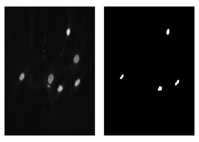
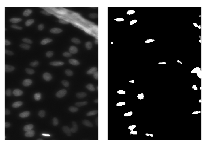
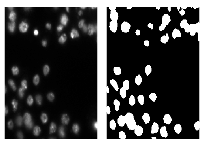
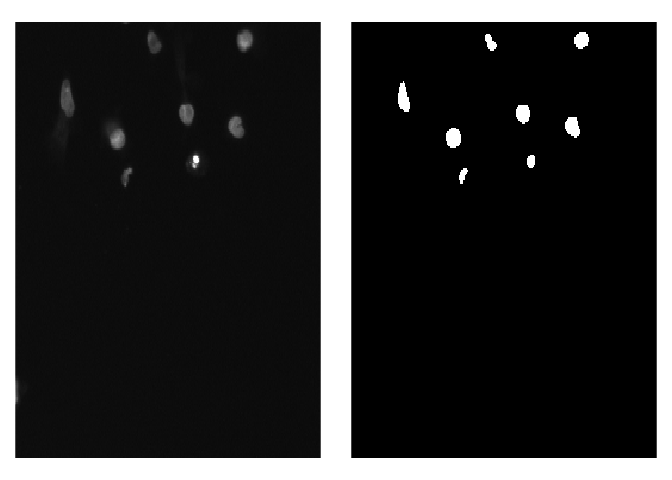
To visualize predicted masks with the original images you can use plot_masks function.

test_imgs_paths <- create_images_masks_paths(test_path, "nested_dirs", FALSE, c("images", "masks"), ";")$images_paths

plot_masks(
  images_paths = test_imgs_paths[1:4],
  masks = test_masks[1:4],
  labels = c("background", "nuclei"),
  colormap = binary_colormap
)